 Many office workers feel like they live in Microsoft Excel, spending hours using spreadsheets to enter data and crunch numbers. By taking advantage of tools like Excel’s freeze feature, workers can make the most of their time by navigating a spreadsheet more efficiently.
Once a spreadsheet grows to be larger than the screen, it can become tricky to navigate. It can be maddening to try and cross-reference a certain row or column on one side of the spreadsheet with another that’s offscreen.
Excel’s freeze feature resolves this pain point by freezing a selected row or column into place, allowing you to scroll off screen while having your needed row or column locked into place. When you think about it, this Excel feature is kind of like a grown-up version of freeze tag.
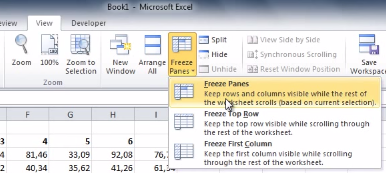
To freeze a row or column in Excel, select the cell that’s in the first column and row that you don’t want to be frozen. Next, go to the View tab and click Freeze Panes. A drop down menu will appear. From here, click on the first option, Freeze Panes.
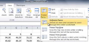
With your selected rows now frozen in place, you will be able to scroll up, down, and sideways in your spreadsheet without having your needed columns or rows move off screen. When you’re ready to unfreeze your rows and columns, simply select any row or column and then go to the View tab. Now go to Freeze Panes > Unfreeze Panes.
This is just one of the many Microsoft Office features that make navigating a project easier. Be sure to check back next week for more time-saving technology tips.